Can You First Check Whether There Are Nans Then Drop Them and Draw the Map Again

Exploratory Data Analysis(EDA): Python

Learning the basics of Exploratory Data Analysis using Python with Numpy, Matplotlib, and Pandas.

Photo by UX Indonesia on Unsplash

What is Exploratory Data Analysis(EDA)?

If we want to explain EDA in simple terms, it means trying to understand the given data much better, so that we can make some sense out of it.

We can find a more formal definition in Wikipedia .

In statistics, exploratory data analysis is an approach to analyzing data sets to summarize their main characteristics, often with visual methods. A statistical model can be used or not, but primarily EDA is for seeing what the data can tell us beyond the formal modeling or hypothesis testing task.

EDA in Python uses data visualization to draw meaningful patterns and insights. It also involves the preparation of data sets for analysis by removing irregularities in the data.

Based on the results of EDA, companies also make business decisions, which can have repercussions later.

• If EDA is not done properly then it can hamper the further steps in the machine learning model building process.
• If done well, it may improve the efficacy of everything we do next.

In this article we'll see about the following topics:

1. Data Sourcing
2. Data Cleaning
3. Univariate analysis
4. Bivariate analysis
5. Multivariate analysis

1. Data Sourcing

Data Sourcing is the process of finding and loading the data into our system. Broadly there are two ways in which we can find data.

1. Private Data
2. Public Data

Private Data

As the name suggests, private data is given by private organizations. There are some security and privacy concerns attached to it. This type of data is used for mainly organizations internal analysis.

Public Data

This type of Data is available to everyone. We can find this in government websites and public organizations etc. Anyone can access this data, we do not need any special permissions or approval.

We can get public data on the following sites.

• https://data.gov
• https://data.gov.uk
• https://data.gov.in
• https://www.kaggle.com/
• https://archive.ics.uci.edu/ml/index.php
• https://github.com/awesomedata/awesome-public-datasets

The very first step of EDA is Data Sourcing, we have seen how we can access data and load into our system. Now, the next step is how to clean the data.

2. Data Cleaning

After completing the Data Sourcing, the next step in the process of EDA is Data Cleaning. It is very important to get rid of the irregularities and clean the data after sourcing it into our system.

Irregularities are of different types of data.

• Missing Values
• Incorrect Format
• Incorrect Headers
• Anomalies/Outliers

To perform the data cleaning we are using a sample data set, which can be found here.

We are using Jupyter Notebook for analysis.

First, let's import the necessary libraries and store the data in our system for analysis.

Now, the data set looks like this,

Marketing Analysis Dataset

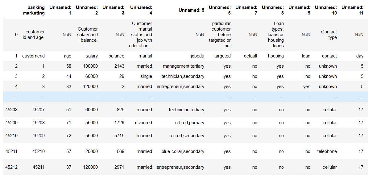
If we observe the above dataset, there are some discrepancies in the Column header for the first 2 rows. The correct data is from the index number 1. So, we have to fix the first two rows.

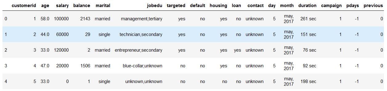
This is called Fixing the Rows and Columns. Let's ignore the first two rows and load the data again.

Now, the dataset looks like this, and it makes more sense.

Dataset after fixing the rows and columns

Following are the steps to be taken while Fixing Rows and Columns:

1. Delete Summary Rows and Columns in the Dataset.
2. Delete Header and Footer Rows on every page.
3. Delete Extra Rows like blank rows, page numbers, etc.
4. We can merge different columns if it makes for better understanding of the data
5. Similarly, we can also split one column into multiple columns based on our requirements or understanding.
6. Add Column names, it is very important to have column names to the dataset.

Now if we observe the above dataset, the customerid column has of no importance to our analysis, and also the jobedu column has both the information of job and education in it.

So, what we'll do is, we'll drop the customerid column and we'll split the jobedu column into two other columns job and education and after that, we'll drop the jobedu column as well.

Now, the dataset looks like this,

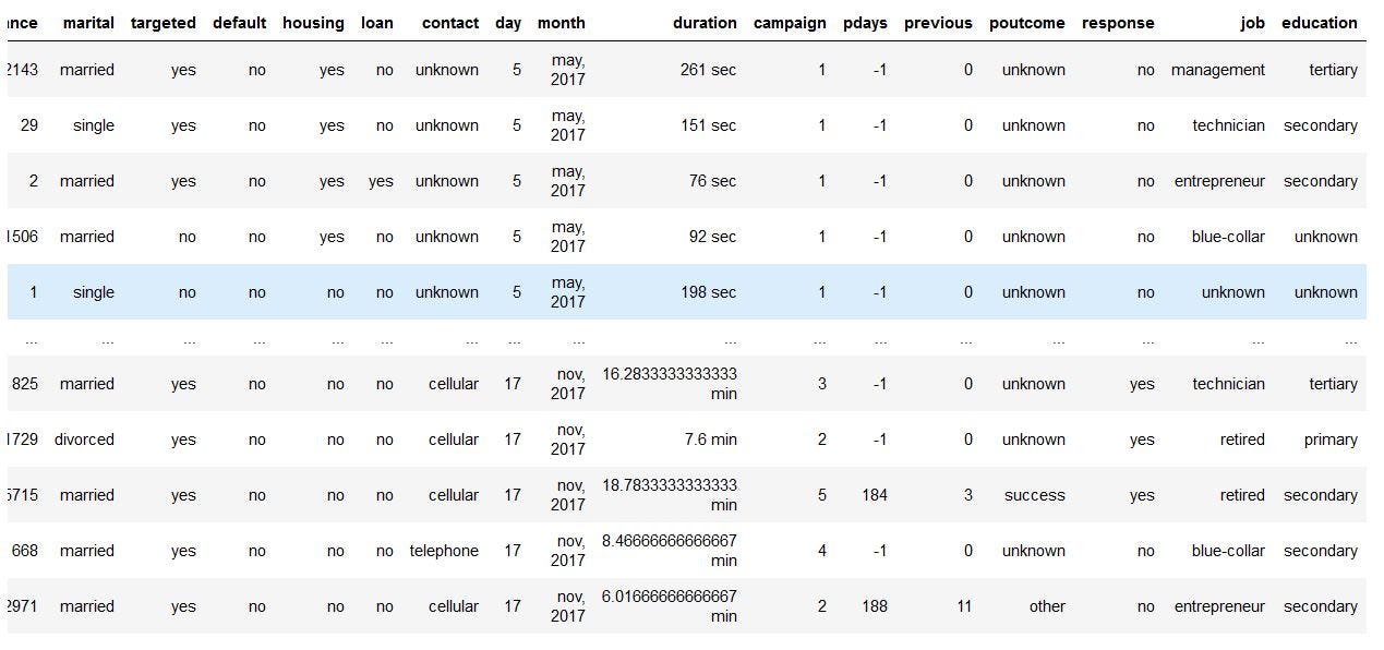
Dropping Customerid and jobedu columns and adding job and education columns

Missing Values

If there are missing values in the Dataset before doing any statistical analysis, we need to handle those missing values.

There are mainly three types of missing values.

1. MCAR(Missing completely at random): These values do not depend on any other features.
2. MAR(Missing at random): These values may be dependent on some other features.
3. MNAR(Missing not at random): These missing values have some reason for why they are missing.

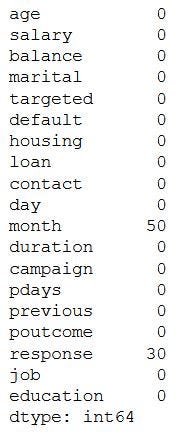
Let's see which columns have missing values in the dataset.

          # Checking the missing values
data.isnull().sum()        

The output will be,

Null Values in Data Set

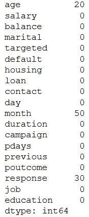
As we can see three columns contain missing values. Let's see how to handle the missing values. We can handle missing values by dropping the missing records or by imputing the values.

Drop the missing Values

Let's handle missing values in the age column.

Let's check the missing values in the dataset now.

Missing Values after handling age column

Let's impute values to the missing values for the month column.

Since the month column is of an object type, let's calculate the mode of that column and impute those values to the missing values.

Now output is,

          # Mode of month is
            'may, 2017'                    # Null values in month column after imputing with mode
            0                  

Handling the missing values in the Response column. Since, our target column is Response Column, if we impute the values to this column it'll affect our analysis. So, it is better to drop the missing values from Response Column.

          #drop the records with response missing in data.
            data = data[~data.response.isnull()].copy()                    # Calculate the missing values in each column of data frame
            data.isnull().sum()                  

Let's check whether the missing values in the dataset have been handled or not,

All the missing values have been handled

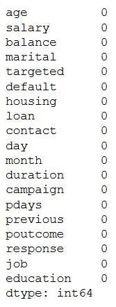
We can also, fill the missing values as 'NaN' so that while doing any statistical analysis, it won't affect the outcome.

Handling Outliers

We have seen how to fix missing values, now let's see how to handle outliers in the dataset.

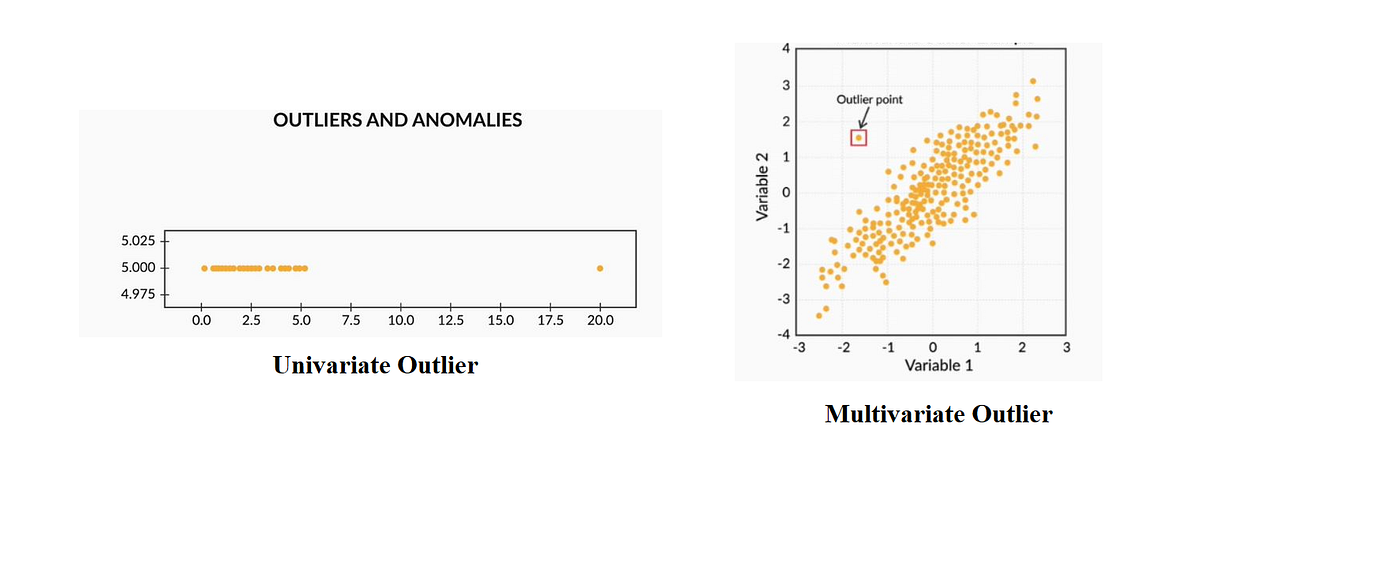
Outliers are the values that are far beyond the next nearest data points.

There are two types of outliers:

1. Univariate outliers: Univariate outliers are the data points whose values lie beyond the range of expected values based on one variable.
2. Multivariate outliers: While plotting data, some values of one variable may not lie beyond the expected range, but when you plot the data with some other variable, these values may lie far from the expected value.

So, after understanding the causes of these outliers, we can handle them by dropping those records or imputing with the values or leaving them as is, if it makes more sense.

Standardizing Values

To perform data analysis on a set of values, we have to make sure the values in the same column should be on the same scale. For example, if the data contains the values of the top speed of different companies' cars, then the whole column should be either in meters/sec scale or miles/sec scale.

Now, that we are clear on how to source and clean the data, let's see how we can analyze the data.

3. Univariate Analysis

If we analyze data over a single variable/column from a dataset, it is known as Univariate Analysis.

Categorical Unordered Univariate Analysis:

An unordered variable is a categorical variable that has no defined order. If we take our data as an example, the job column in the dataset is divided into many sub-categories like technician, blue-collar, services, management, etc. There is no weight or measure given to any value in the 'job' column.

Now, let's analyze the job category by using plots. Since Job is a category, we will plot the bar plot.

The output looks like this,

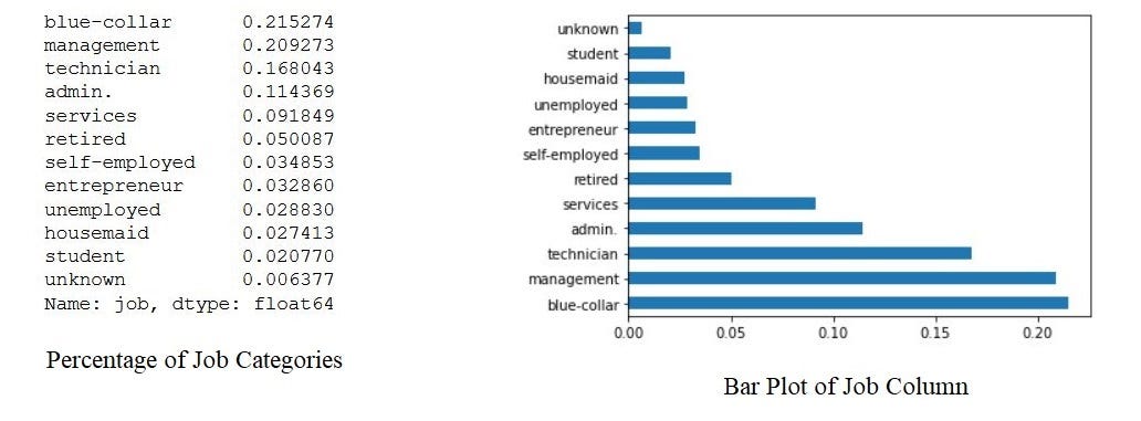
By the above bar plot, we can infer that the data set contains more number of blue-collar workers compared to other categories.

Categorical Ordered Univariate Analysis:

Ordered variables are those variables that have a natural rank of order. Some examples of categorical ordered variables from our dataset are:

• Month: Jan, Feb, March……
• Education: Primary, Secondary,……

Now, let's analyze the Education Variable from the dataset. Since we've already seen a bar plot, let's see how a Pie Chart looks like.

The output will be,

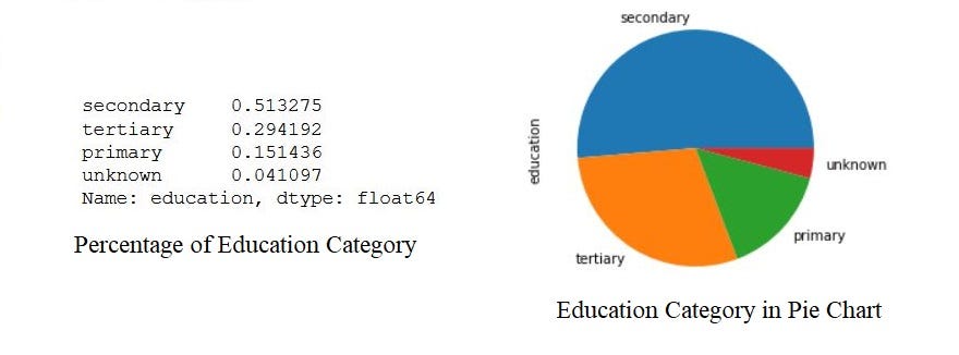
By the above analysis, we can infer that the data set has a large number of them belongs to secondary education after that tertiary and next primary. Also, a very small percentage of them have been unknown.

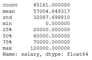
This is how we analyze univariate categorical analysis. If the column or variable is of numerical then we'll analyze by calculating its mean, median, std, etc. We can get those values by using the describe function.

          data.salary.describe()        

The output will be,

4. Bivariate Analysis

If we analyze data by taking two variables/columns into consideration from a dataset, it is known as Bivariate Analysis.

a) Numeric-Numeric Analysis:

Analyzing the two numeric variables from a dataset is known as numeric-numeric analysis. We can analyze it in three different ways.

• Scatter Plot
• Pair Plot
• Correlation Matrix

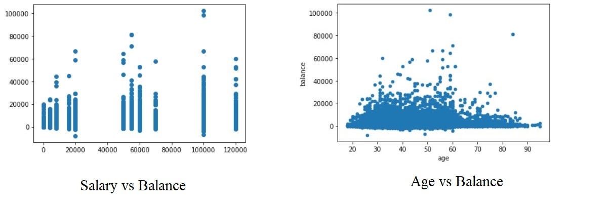
Scatter Plot

Let's take three columns 'Balance', 'Age' and 'Salary' from our dataset and see what we can infer by plotting to scatter plot between salary balance and age balance

Now, the scatter plots looks like,

Scatter Plots

Pair Plot

Now, let's plot Pair Plots for the three columns we used in plotting Scatter plots. We'll use the seaborn library for plotting Pair Plots.

The Pair Plot looks like this,

Pair Plots for Age, balance, Salary

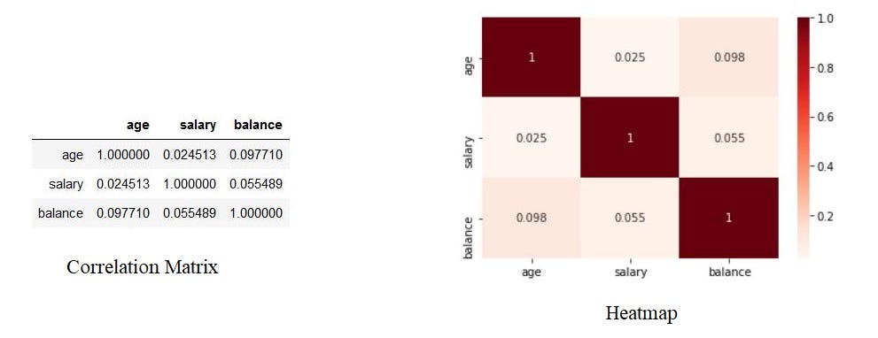
Correlation Matrix

Since we cannot use more than two variables as x-axis and y-axis in Scatter and Pair Plots, it is difficult to see the relation between three numerical variables in a single graph. In those cases, we'll use the correlation matrix.

First, we created a matrix using age, salary, and balance. After that, we are plotting the heatmap using the seaborn library of the matrix.

b) Numeric - Categorical Analysis

Analyzing the one numeric variable and one categorical variable from a dataset is known as numeric-categorical analysis. We analyze them mainly using mean, median, and box plots.

Let's take salary and response columns from our dataset.

First check for mean value using groupby

          #groupby the response to find the mean of the salary with response no & yes separately.                      data.groupby('response')['salary'].mean()                  

The output will be,

Response and Salary using mean

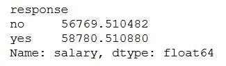
There is not much of a difference between the yes and no response based on the salary.

Let's calculate the median,

          #groupby the response to find the median of the salary with response no & yes separately.                      data.groupby('response')['salary'].median()                  

The output will be,

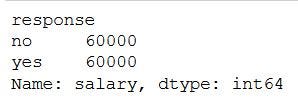
By both mean and median we can say that the response of yes and no remains the same irrespective of the person's salary. But, is it truly behaving like that, let's plot the box plot for them and check the behavior.

          #plot the box plot of salary for yes & no responses.                      sns.boxplot(data.response, data.salary)
plt.show()                  

The box plot looks like this,

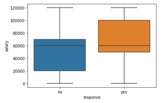
As we can see, when we plot the Box Plot, it paints a very different picture compared to mean and median. The IQR for customers who gave a positive response is on the higher salary side.

This is how we analyze Numeric-Categorical variables, we use mean, median, and Box Plots to draw some sort of conclusions.

c) Categorical — Categorical Analysis

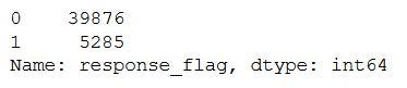
Since our target variable/column is the Response rate, we'll see how the different categories like Education, Marital Status, etc., are associated with the Response column. So instead of 'Yes' and 'No' we will convert them into '1' and '0', by doing that we'll get the "Response Rate".

The output looks like this,

Let's see how the response rate varies for different categories in marital status.

The graph looks like this,

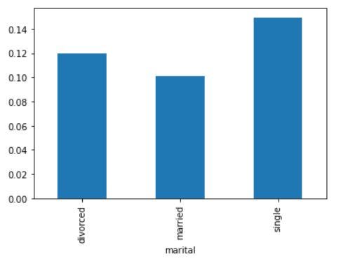
By the above graph, we can infer that the positive response is more for Single status members in the data set. Similarly, we can plot the graphs for Loan vs Response rate, Housing Loans vs Response rate, etc.

5. Multivariate Analysis

If we analyze data by taking more than two variables/columns into consideration from a dataset, it is known as Multivariate Analysis.

Let's see how 'Education', 'Marital', and 'Response_rate' vary with each other.

First, we'll create a pivot table with the three columns and after that, we'll create a heatmap.

The Pivot table and heatmap looks like this,

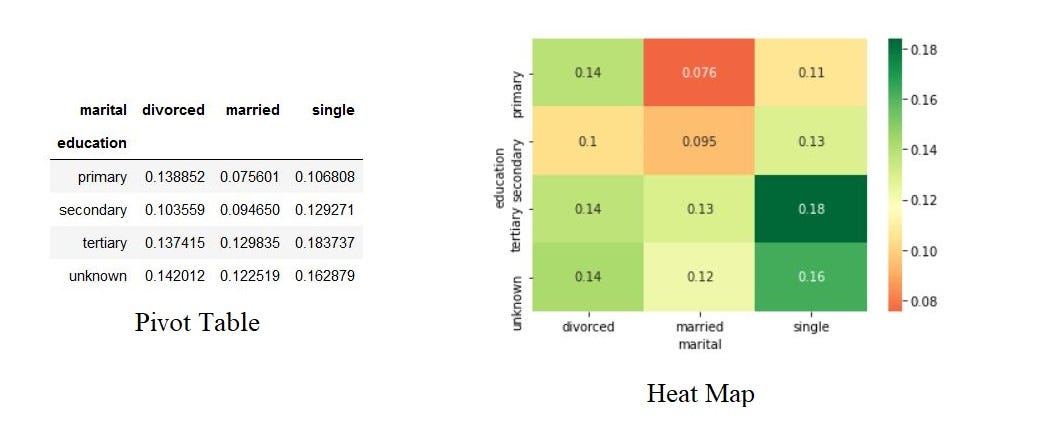
Based on the Heatmap we can infer that the married people with primary education are less likely to respond positively for the survey and single people with tertiary education are most likely to respond positively to the survey.

Similarly, we can plot the graphs for Job vs marital vs response, Education vs poutcome vs response, etc.

Conclusion

This is how we'll do Exploratory Data Analysis. Exploratory Data Analysis (EDA) helps us to look beyond the data. The more we explore the data, the more the insights we draw from it. As a data analyst, almost 80% of our time will be spent understanding data and solving various business problems through EDA.

Thank you for reading and Happy Coding!!!

Check out my previous articles about Python here

• Indexing in Pandas Dataframe using Python
• Seaborn: Python
• Pandas: Python
• Matplotlib: Python
• NumPy: Python
• Data Visualization and its Importance: Python
• Time Complexity and Its Importance in Python
• Python Recursion or Recursive Function in Python

References

• Exploratory data analysis: https://en.wikipedia.org/wiki/Exploratory_data_analysis
• Python Exploratory Data Analysis: https://www.datacamp.com/community/tutorials/exploratory-data-analysis-python
• Exploratory Data Analysis using Python: https://www.activestate.com/blog/exploratory-data-analysis-using-python/
• Univariate and Multivariate Outliers: https://www.statisticssolutions.com/univariate-and-multivariate-outliers/

wilsonyouslovis.blogspot.com

Source: https://towardsdatascience.com/exploratory-data-analysis-eda-python-87178e35b14

Share this post